Rocket Experiment for Neutral Upwelling 2
NASA Mission 52.002 - Flight Data & Results
On this page you will find data and/or basic plots that have been superceded by newer or more relevant information:
Data & Plot Archive
52.002 Lessard - Preliminary Attitude Solution |
| Main Payload Attitude |
Data files:
Data in .csv format
GPS Main in .dat
Mag Vec in .dat |
T0: 12\13\2015 7:34:0.7 GMT
Launcher Settings: Lat = 69.2942 Deg., Lon. = 16.0193 Deg.
Alt: 171.3 Ft, El: 80.28 Deg., Az: 12.08 Deg., Bank: 0 Deg.
Attitude Output: time (sec from T0), roll (Euler angle in deg.), yaw, pitch, Roll rate, Euler angle matrix elements, local geodetic coordinates and velocity of the payload, lat (geo), long (Geo), Altitude(meters)
Position Source: GPS
Attitude Source: GLNMAC
See the README file for further detail on the file contents
|
| UNH UV PMT Data Plot (Andoya TM) (Bruce Fritz, 5 January 2016) |

|
UV PMT data is a plot of counts vs time. Time resolution is 1 ms. The blue trace is the raw data. The black trace is a smoothed version of the raw data using a 100-pt boxcar smooth function
The UV PMT measures neutral atomic oxygen density variations ABOVE the payload by measuring sunlight scattered from the atoms. It was included on the payload following a suggestion from Dirk Lummerzheim, but is not a calibrated instrument. Moving forward, it is our intention to replicate the UV PMT and to calibrate an "identical" instrument in order to estimate the brightness in Rayleighs. The data appear to be excellent and seem to show enhanced oxygen densities in the region of electron precipitation, as hoped for. Before T+455 or so, there is no significant precipitation and we believe that the signal strength dropped below the noise floor of the PMT.
|
| EPLAS Quick-look summary plot (Andoya TM) (Mark Widholm, 16 December 2015) |

|
Should have the correct time scale in sec after T-0. Looks like HV on is at about T+233. .RC1 file ends at T+660
Highest intensity is between T+580 and T+590 and is about 5 MHz event rate with dead-time correction. This pushes the saturation limit but looks ok.
Angular distribution (HEI) data also looks good but doesn't lend itself to a summary-type plot. Intense low energy stuff after 440 generally shows as field aligned but here is variation with energy and time. Will work on other meaningful plots
EPLAS housekeeping monitors were nominal for entire flight
|
| Pitch Angle Distribution Plots (Andoya TM) (Mark Widholm, 6 January 2015) |

|

|
This info is a little out of date but was the first look at the 2 keV mystery signal.
These plots assign pitch angle based on the pad look direction and do not correct for the actual payload motion. A crude check of payload alignment based on magnetometer data shows ~2 deg coning and a worst case misalignment of 12 deg. Since the angle pads are 10 deg wide, the payload motion would change things a little but it would not be a large effect. The detector angle pads cover a full 360 deg so these pitch angle bins are the average of two pads when available. There are blind spots so some pitch angles only have data from one pad.
The low energy, high intensity bursts are field aligned. The high energy stuff early in the flight is a mixture of field aligned and spread out to 90 deg. The log intensity scale and averaging tends to obscure the fact that the highest flux is near 0 deg (electrons moving straight down the field) but it allows you to see what is happening over a wide range of intensity.
In the region from about T0+565 to 605 where the energy spectra show the flat top at about 2KeV, the angular distribution clearly shows the 2KeV population coming from below 90 deg and moving up the field. The sharp edges look a bit unnatural, but housekeeping monitors etc. show no evidence that the instrument was doing anything differently at the time.
The 2KeV stuff is bursty and not there on every energy sweep. It does not appear to be very directly correlated with the timing of low energy bursts.
|
| Main Payload Pitch Angle (Mark Widholm, 6 January 2016) |

|
The Cornell science magnetometer data is plotted as a proxy for the pitch angle relative to the local field line. The large trend shows the effect of the predictive field alignment. The shorter time-scale variations are due to a slight coning efffect.
|
HEEPS-M - Higher energy ion instrument |
Flux Data:
|
TBD |
| Quick-look summary plot (Svalbard TM) (Mark Widholm, 21 January 2016) |

|
Data presented here is on the same time scale as the EPLAS instrument. Starts at 230 sec, just before HV turn on at 230 sec and continues at 1 ms intervals through LOS.
Summary plot for high energy ions is presented here.
|
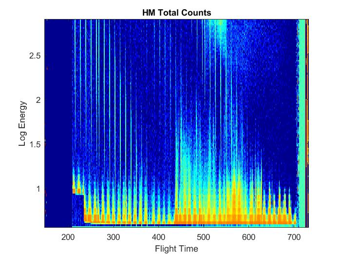 | Summary plot, Meghan Harrington, 9 March 2016 |
HEEPS-T - Thermal Ion Instrument |
Flux Data:
|
TBD |
| Quick-look summary plot (Svalbard TM) (Mark Widholm, 21 January 2016) |

|
Data presented here is on the same time scale as the EPLAS instrument. Starts at 230 sec, just before HV turn on at 230 sec and continues at 1 ms intervals through LOS.
Summary plot for thermal ions is presented here.
|
| UNH UV PMT Data Plot (Andoya TM) (Bruce Fritz, 5 January 2016) |
|
|
UV PMT data is a plot of counts vs time. Time resolution is 1 ms. The blue trace is the raw data. The black trace is a smoothed version of the raw data using a 100-pt boxcar smooth function
The UV PMT measures neutral atomic oxygen density variations ABOVE the payload by measuring sunlight scattered from the atoms. It was included on the payload following a suggestion from Dirk Lummerzheim, but is not a calibrated instrument. Moving forward, it is our intention to replicate the UV PMT and to calibrate an "identical" instrument in order to estimate the brightness in Rayleighs. The data appear to be excellent and seem to show enhanced oxygen densities in the region of electron precipitation, as hoped for. Before T+455 or so, there is no significant precipitation and we believe that the signal strength dropped below the noise floor of the PMT.
|
EISCAT |
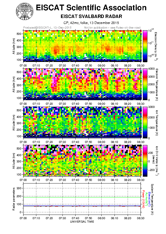
| 42m EISCAT Plot produced immediately after launch (Kjellmar Oksavik, 13 December 2015) |
|
EISCAT data for this event should be reliable up to at least 400 km where electron density begins to fall off.
PMAFs are seen as enhancements in electron temp, starting from 0720 UT onwards. Some are also associated with electron density enhancements in the F-region
There are two brief intervals of strong Joule heating (high ion temp) around 0740 UT and 0745 UT, close to apogee. Suspect significant flow shears, or flow bursts associated with PMAFs. There are often Reversed Flow Events near PMAFs and it would be very exciting to see if there is lots of structure in the E-field, indicative of flow reversals.
Last panel shows ion upflow from 0740-0748 UT in 300-400 km altitude, where data should be reliable.
|
COWBOY - Electric Fields |
Field Data:
|
TBD |
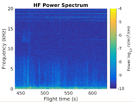
| Preliminary field plots (Dave Hysell, 11 February 2016) |
 |
Data here is still very preliminary and has been analyzed without attitude estimates.
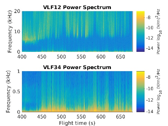
The top plot is HF data in spectrogram format from one of the baselines.
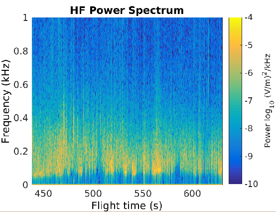
Below that is a zoomed in plot of the top plot with an upper limit of 1 kHz on the frequency axis.
You can find .pdf files for two different time spans:
300s - 500s
450s - 650s
.eps files are available by clicking on the images
The next plot is HF data in spectrogram format from one of the baselines. The middle plot is a zoomed in plot of the top plot with an upper limit of 1 kHz on the frequency axis.
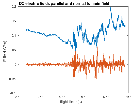
The bottom plot ("v42-21.eps") shows the results of fitting the fields to sine waves. The blue and orange curves are the amplitudes of the fields in phase and in quadrature with the sine-wave fits. The fields are mainly V x B during the first half of the flight but much more active in the second.
.eps files are available by clicking on the images
|
U. Oslo All Sky Imager |
|
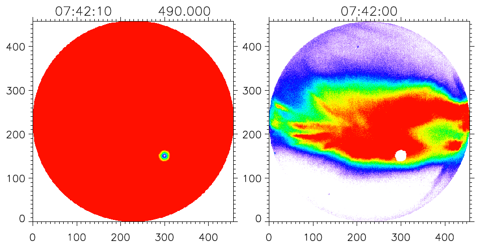
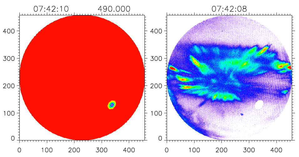
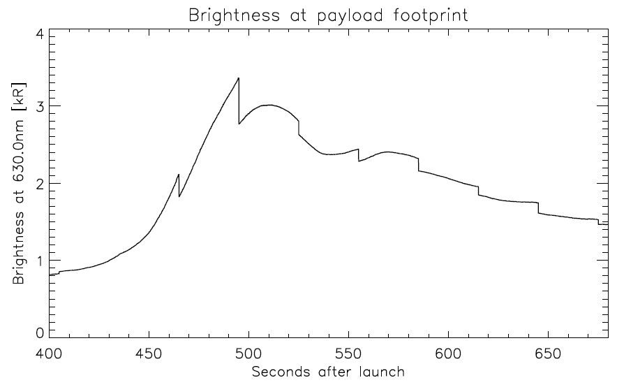
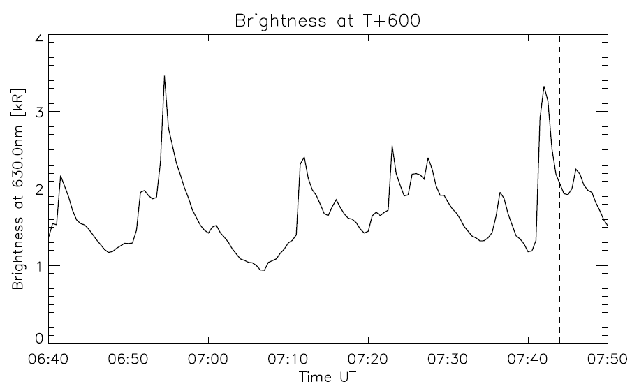
The plots to the left show, for both the 5577 and 6300 nm channel the brightness at the footpoint of the payload and a time series of the brightness at the payload's location at T+600s.
The first two plots to the left a sanity check: it shows for both the 5577 and 6300 nm channel the distance between the location of each ASI pixel (on the left, mapped to 250 km altitude for 6300 nm and mapped to 150 km altitude for 5577 nm) and the payload. I chose the color scale such that all distances greater than 20 km are red. Essentially, then, the plot shows through the eyes of the ASI where the payload was located. On the right I show the actual ASI image. All pixels within a 20 km radius around the payload are white in this plot. Those are the values that I include when calculating the brightness at the payload footprint. Remember that I not only map the ASI data to altitude, I also map the payload location to that same altitude using IGRF.
Note that the payload is closer to the edge of the 5577 nm image because that is mapped to 150 km altitude, whereas the 6300 nm data is mapped to 250 km altitude, making the field-of-view larger.
I know that the plots do not include axis labels and color bars - I hope you can forgive me breaking the Second Commandment of experimental physics "Thou shall never produce plots without proper labeling" since these are only meant as sanity checks.
The third plot than shows the brightness at the payload footprint for the 630.0 nm channel only. Each time a step occurs is because the data is now extracted from a new ASI image - the time resolution of the 5577 nm images is 15 seconds, that of the 630.0 nm images is 30 seconds.
The last plot is the brightness in the region 20 km around the payload location at T+600s as a function of time, also only for the 630.0 nm channel.
Example plots can be found here for:
557.7 nm data
630.0 nm data
|
| Imager Summary Plots (Lasse Clausen, 19 January 2016)
|
| For 5577 summary plots, click here. |
|
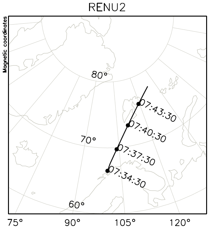
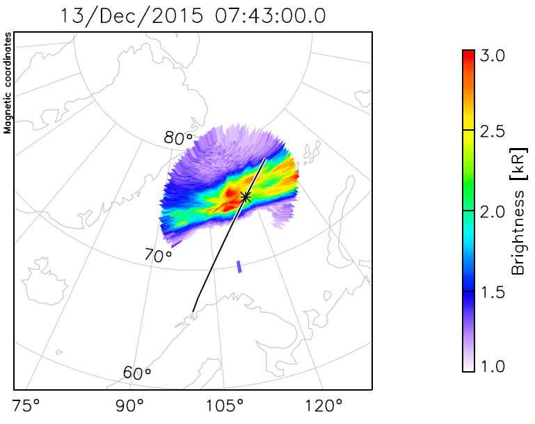
Example plots of the rocket trajectory plotted with the ASI observations from Longyearbyen at 6300 \C5. Rocket footprint is along the IGRF to 250 km altitude. Click on the plots to open the full file of plots:
1) Trajectory (mapped to altitude) in AACGM coordinates (left, top)
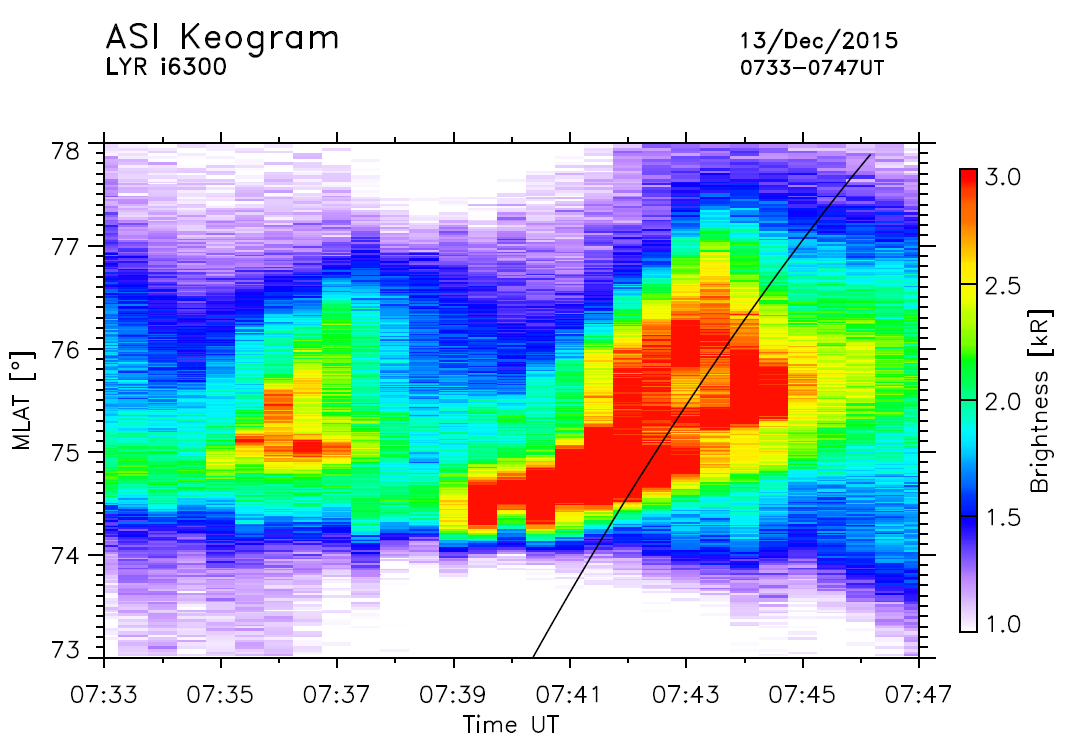
2) Overview keogram along magnetic meridian
3) Zoom keogram with the rocket latitude overlaid (left, middle) - note that you cannot really relate the auroral brightnesses and the rocket observations because the rocket does not fly along the magnetic meridian
4) Altitude vs. time plot, colored according to the actual brightness detected by the ASI at the mapped location of the rocket - I made this plot to make sure that when the rocket crossed the intense 6300 \C5 emissions, it was most probably above the emissions, i.e., where you would expect the upwelling
5) One plot every minute (left, bottom) showing the mapped rocket location and the ASI observations (also marked by vertical dashed line in the time vs. altitude plot)
From these data is seems like the rocket was exactly in the right location to observe upwelling due to soft particle precipitation that started 0739 UT
Our imager has a resolution of 20-30 seconds; I can prepare plots of all the images we have during the flight. Note that these images are already available (click your way to the right date, and chose the appropriate hour of the Longyearbyen keogram - below it is a link "show individual images" which does just that) However, these images are individually scaled so it is difficult to compare between them - like I said, I will prepare all images on a common scale for you. You can also download the PNGs from the website and do your own analysis (click "open raw image folder" instead of "show individual images").
|
|